3GPP Rel-19 introduces a new standardized approach for modeling 6G UT antennas in 3GPP channel. This post explains the procedure step by step, from radiation patterns to polarization, with reproducible Python examples.
New antenna modeling was introduced in 3GPP Release-19 as part of the channel-modeling study. For background on the channel model update itself, see my earlier post: 7–24 GHz channel model.
In this post, I take a closer look at the standardized procedure for calculating User Terminal (UT) antenna radiation patterns and polarization components, as specified in Clause 7.3 “Antenna Modelling” of the updated Rel-19 TR 38.901.
All figures presented here are generated using Python code that follows the TR specification. The full code is available on GitHub:
6g_ue_antennas.
At the moment, the repository includes:
antenna.ipynb: a Jupyter notebook for plotting antenna radiation patterns.
utils.py: a Python module that implements the transformation logic and plotting functions.
In the sections below, I walk through each step of UT antenna modeling and illustrate it using the shared Python code.
Before Rel-19, UT antennas were modeled in a simplified way: as two (or more) cross-polarized components with omnidirectional radiation patterns. Antenna elements were typically spaced half a wavelength \( \lambda/2 \) apart—for example, four transmit antennas on the UT side might be arranged in a simple X X configuration.
The new model introduces directional radiation patterns, as defined in Table 7.3-2 of TR 38.901. In this model, the antenna is assumed to be oriented toward \( \theta^{\prime\prime}=90^\circ \) and \( \phi^{\prime\prime}=0^\circ \).
Table 1: Radiation power pattern of a single antenna element for handheld UT (Table 7.3-2 from TR 38.901)
Maximum directional gain of an antenna element \( G_{E,\max} \)
5.3 dBi
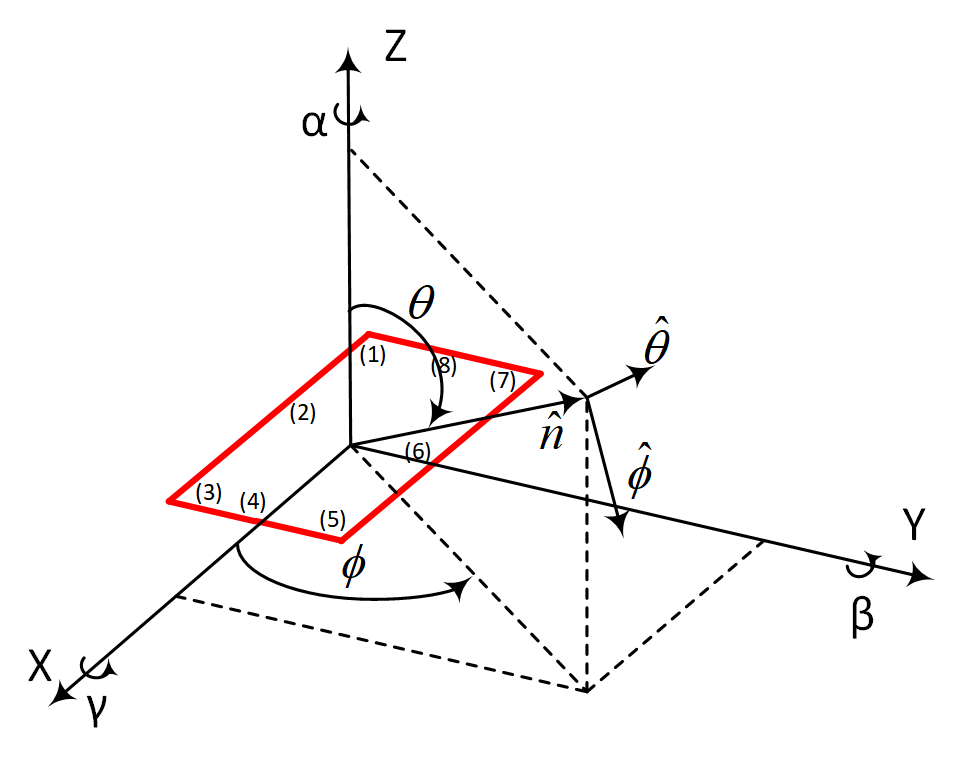
The angles \( \theta'' \) and \( \phi'' \) denote zenith/elevation and azimuth, respectively. Their definitions follow Figure 7.1.1 in TR 38.901 and are reproduced below.
Figure 1: Definition of spherical angles, spherical unit vectors, 3D rotation angles, and reference UT orientation in a Cartesian coordinate system.
\( \hat{\theta} \) and \( \hat{\phi} \) are unit vectors forming an orthogonal basis for each signal arrival/departure direction \( \hat{n} \) associated with angles \( (\theta,\phi) \). The double primes used for the angles and the reference radiation pattern \( A''_{dB}(\theta'',\phi'') \) refer to the reference Antenna Coordinate System (ACS), \( (x'',y'',z'',\theta'',\phi'') \). The radiation pattern at each candidate UT antenna location can be defined in a Local Coordinate System (LCS), denoted with single primes, \( (x',y',z',\theta',\phi') \). A Global Coordinate System (GCS) is used for scenarios involving multiple BSs and UTs and is written without primes, \( (x,y,z,\theta,\phi) \).
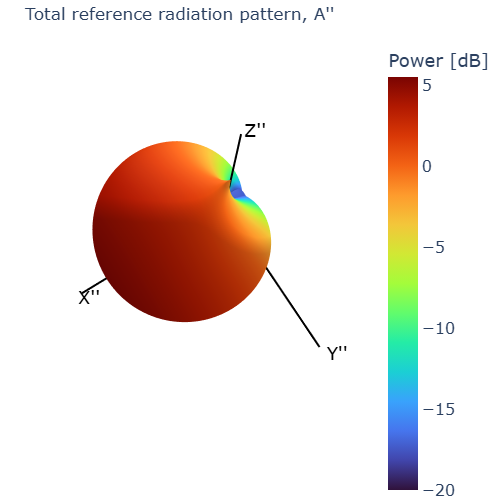
The parameters of the reference radiation pattern (shown below) are defined in utils.py in the dictionary RADIATION_PATTERN_DEFAULTS.
Figure 2: Radiation power pattern of a single reference antenna element for handheld UT, \( A''_{dB}(\theta'', \phi'') \).
Antenna candidate locations
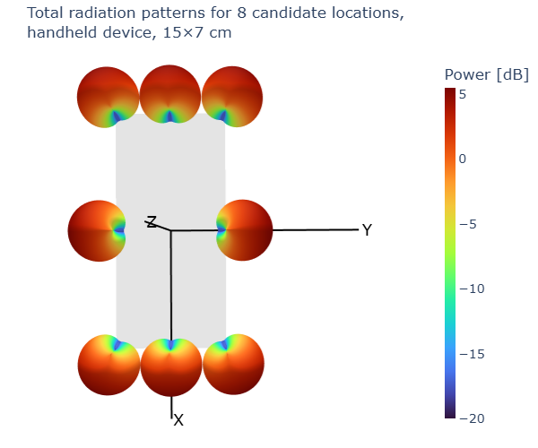
3GPP adopted reference device dimensions of 55 × 7 × 0 mm for handheld UTs. Based on this, eight candidate antenna locations were identified: four at the corners and four at the midpoints of the device edges. For each location, the maximum-gain direction is aligned with the axis pointing from the device center to that location. Accordingly, the reference radiation pattern is rotated and translated to each candidate position. The resulting patterns are shown below.
Figure 3: Radiation power patterns for all UT candidate antenna locations (top-down view).
Antenna polarization
UT antenna polarization is more complex than for BS because real UT antennas are usually single-feed elements that do not produce a purely vertically or horizontally polarized wave. Instead, the polarization varies with direction and often results in an elliptically polarized field.
The general relationship between the radiation field and the power pattern is:
$$
A''(\theta'',\phi'') = \bigl|F''_{\theta''}(\theta'',\phi'')\bigr|^2 + \bigl|F''_{\phi''}(\theta'',\phi'')\bigr|^2 .
$$
Here, \( F''_{\theta} \) is the field component along \( \hat{\theta}'' \), and \( F''_{\phi} \) is the component along \( \hat{\phi}'' \).
Earlier versions of TR 38.901 already included two polarization modeling options (as also described in the paper 3D Channel Model in 3GPP):
Model-1: a slanted dipole polarization model. This model is based on the idea that a polarization slant \( \zeta \) can be modelled as a mechanical tilt. This model achieves equal power split in vertical and horizontal directions at the antenna boresight, but the power split ratio depends on both azimuth and elevation direction \( \theta, \phi \).
Model-2: a constant/angle-independent polarization model. This model assumes that the polarization power split is independent of azimuth and elevation angles \( \theta, \phi \). Considering a \( \zeta=\pm45^\circ \) cross-polarized transmit antenna pair, the constant polarization model assumption leads to an equal power split in vertical and horizontal for all signal directions around the antenna.
For UT antennas, a Model-1-like approach is adopted: polarization depends on the departure/arrival direction and on the antenna/UT orientation. The UT reference radiation pattern is assumed vertically polarized, with all gain in the \( \theta \) component:
$$
F''_{\theta''}(\theta'',\phi'') = \sqrt{A''(\theta'',\phi'')}, \quad F''_{\phi''}(\theta'',\phi'') = 0 .
$$
First step. Rotate each polarized field component of the reference pattern, \( F''_{\theta''}(\theta'',\phi'') \) and \( F''_{\phi''}(\theta'',\phi'') \), according to the orientation and polarization direction of each UT antenna \( u \). This yields the rotated components \( F'_{u,\theta'}(\theta',\phi') \) and \( F'_{u,\phi'}(\theta',\phi') \), using the coordinate-transformation formulas in Clause 7.1.3 of TR 38.901:
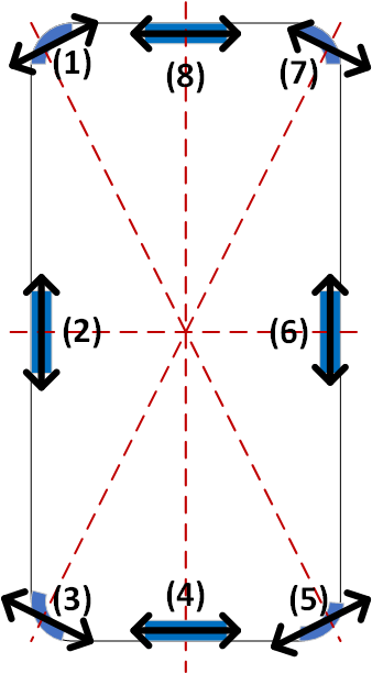
The rotation angles (\(\alpha_u,\beta_u,\gamma_u\)) are derived from each antenna’s orientation and polarization direction in the LCS. Figure 4 illustrates these orientations: the bold arrows lie in the plane of the handheld device and are perpendicular to the axis connecting the device center to each candidate antenna location.
Figure 4: Handheld UT antenna polarization directions for one antenna field pattern (top down view), (Figure 7.3-7 from TR 38.901).
The reference pattern, polarized along \( Z'' \), must therefore be rotated to align with these indicated directions. The table below lists the corresponding 3D rotation angles for each candidate antenna.
Table 2: 3D rotation angles per candidate antenna
\(\alpha_u\)
\(\beta_u\)
\(\gamma_u\)
Antenna #
-155°
0°
90°
1
-90°
0°
90°
2
-25°
0°
90°
3
0°
0°
90°
4
25°
0°
90°
5
90°
0°
90°
6
155°
0°
90°
7
180°
0°
90°
8
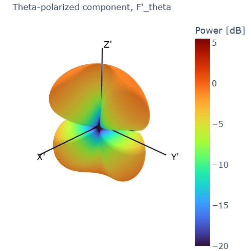
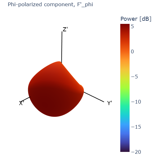
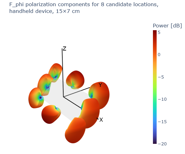
The provided Jupyter notebook can generate 3D plots of the total radiation pattern and the polarization components for each antenna. For example, Figures 5–7 show the total power,\( \theta \)-polarized component, and \( \phi\)-polarized component for Antenna 5.
Figure 5: Radiation power pattern for UT antenna (5).Figure 6: \( F_{5,\theta} \) polarization component for UT antenna (5).Figure 7: \( F_{5,\phi} \) polarization component for UT antenna (5).
Once the antenna-level rotation is applied, in the second step, the resulting polarized components \( F'_{u,\theta'}(\theta',\phi') \) and \( F'_{u,\phi'}(\theta',\phi') \) must be rotated again according to the orientation of the UT in the global coordinate system (GCS). This step uses the rotation angles defined in Clause 7.1.3 of TR 38.901. The following equations, similar to (7.1-11), (7.1-7), (7.1-8), (7.1-16), and (7.1-17) from Clause 7.1.3 of TR 38.901, are used to perform the transformations.
Table 3: 3D rotation angles per typical UT orientations
UT orientation
\( \Omega_{\text{UT},\alpha} \)
\( \Omega_{\text{UT},\beta} \)
\( \Omega_{\text{UT},\gamma} \)
One-hand hold/blockage
0–360°
45°
0°
Dual-hand hold/blockage
0–360°
0°
45°
Hand hold and head blockage
0–360°
90°
0°
Free space browsing
0–360°
45°
0°
Horizontal on the surface
0–360°
0°
0°
It is worth noting that the two-step rotation procedure (antenna-level rotation followed by UT-level rotation) can be combined into a single equivalent rotation. However, the resulting angles differ from those applied in the two-step approach. For example, for antenna (6) in the free space browsing case, the two-step sequence is \( (\alpha_6=90^\circ, \beta_6=0^\circ, \gamma_6=90^\circ) \) followed by \( (\Omega_{\alpha}=0^\circ, \Omega_{\beta}=45^\circ, \Omega_{\gamma}=0^\circ) \). The equivalent single rotation would instead be \( (\alpha=90^\circ, \beta=0^\circ, \gamma=-45^\circ) \).
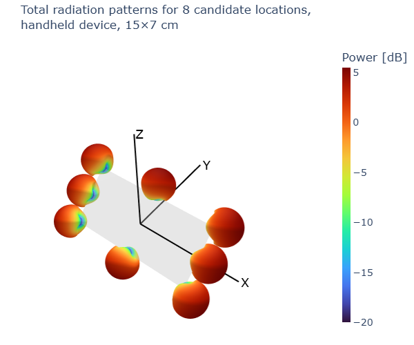
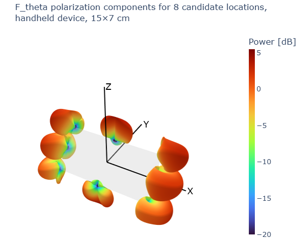
The Jupyter notebook also allows visualization of the polarization components together with the UT orientation. For example, Figures 8–10 show the radiation patterns and polarization components for all candidate antenna locations when the UT is in a dual-hand grip.
Figure 8: Radiation power patterns for all UT candidate antenna locations in dual-hand grip.Figure 9: \( F_{\theta} \) polarization component for all UT candidate antenna locations in dual-hand grip.Figure 10: \( F_{\phi} \) polarization component for all UT candidate antenna locations in dual-hand grip.
Key takeaways
Rel-19 introduces directional UT antenna patterns to replace the earlier simplistic omnidirectional model.
Antenna placement matters: eight candidate locations are standardized on a handheld device, with radiation patterns rotated accordingly.
Polarization is modeled realistically: UT antennas are assumed vertically polarized in the reference pattern, with orientation-dependent transformations applied.
Two rotation steps are required: first at the antenna level (local orientation), then at the device level (UT orientation in GCS). These can also be combined into a single equivalent rotation.
Python code is available: all figures in this post were generated using the 6g_ue_antennas repository, which provides both plotting and transformation utilities.
Найдите идеальный вариант для своего бизнеса и <a href=https://klpl3r.ru/>slm 3d принтер купить|3д принтер slm купить|slm принтер по металлу купить|slm принтер купить</a> уже сегодня!
В интернет-сообществах можно найти ответы на распространенные вопросы.
3d_uopa (2025-10-24 17:57)
<a href=https://metr3s-vd.ru/>3d принтер по металлу купить</a> обеспечивает высокую точность и качество изделий, что делает его идеальным выбором для промышленных потребностей.
3D принтер по металлу — это удивительное устройство, способное revolutionize производство. Каждый год появляется множество инноваций, которые способствуют процесс печати. Технологии 3D печати по металлу все чаще используются в различных отраслях.
Применение 3D печати по металлу открывает новые возможности для дизайнеров. Используя эту технологию, можно производить сложные детали с высокой точностью. В дополнение, процессы стали более эффективными и экономичными. Таким образом, возможно сократить время на производство и снизить затраты.
Процессы 3D печати металла основаны на аддитивном подходе, где каждая деталь добавляется последовательно. Данная технология предоставляет шанс создавать объекты, которые невозможно изготовить другими способами. Важным моментом становится контроль качества на каждом этапе создания детали.
Развитие аддитивных технологий выглядит очень многообещающим. По мере развития технологии совершенствуются, и появляются новые решения. открывает возможности для новых проектов и улучшает существующие. Скоро мы можем ожидать доступности 3D принтеров по металлу на рынке.
Vnedrenie_hvKt (2025-10-24 22:06)
<a href=https://nedr-vcm04.ru/>Внедрение WMS системы</a> значительно улучшает эффективность управления складскими процессами.
Важным аспектом внедрения WMS является обучение персонала.
Georgedof (2025-10-27 16:37)
Hej, jeg ønskede at kende din pris.
Promyshlen_uuea (2025-11-01 22:47)
<a href=https://prbn-sknr1.ru/>3d сканер промышленный купить</a> становятся всё более востребованными в производственной сфере благодаря своей точности и эффективности.
В настоящее время промышленные 3D сканеры являются важным инструментом для высокоточных измерений.
Georgedah (2025-11-18 19:10)
Здравейте, исках да знам цената ви.
AustralianGameNen (2025-11-19 16:57)
Australian Games Fund: learn about government support for gaming industry, grants, and development opportunities at https://australiangames.top/
AustralianGameShowsGor (2025-11-19 19:14)
Game shows function as cultural touchstones documented at https://australiangameshows.top/ creating nostalgic connections enduring decades.
GratiaVitaeGor (2025-11-21 06:29)
Как улучшить общение с родными и близкими — практические рекомендации. https://gratiavitae.ru/
PerplexityKupitGor (2025-11-22 14:37)
perplexity ai pro 1 год https://uniqueartworks.ru/perplexity-kupit.html
MetabolicFreedomGor (2025-11-23 16:23)
Discover how keto fasting, quality sleep, and mindset shifts combine for total metabolic recovery. https://metabolicfreedom.top/ metabolic freedom with ben azadi
cazino_roEa (2025-12-07 05:30)
?Llevas tiempo queriendo encontrar un buen casino online legal en Espana para apostar con dinero real? Yo tambien estuve en esa situacion hasta que encontre <a href=casinos-dinero-real.mystrikingly.com>poker online dinero real espaГ±a</a>.
Este sitio me parecio una comparativa actualizada de casinos en linea en Espana donde los pagos estan garantizados. Lo mas importante para mi fue que todos los casinos tienen licencia oficial. Eso da confianza. Ademas, puedes jugar desde el movil. Yo juego desde Madrid y todo cargo perfectamente.
?Promociones? ?Por supuesto! Los casinos que aparecen en esta web ofrecen recompensas por primer deposito para que empieces con ventaja. ?Prefieres ruleta? La oferta es variada. Desde juegos de mesa en vivo hasta baccarat clasico, todo esta ahi.
Los cobros es rapido. Yo recibi el dinero por transferencia y me llego en 24h. Eso demuestra seriedad. Si eres de Madrid, te aconsejo revisar esta plataforma. Veras sitios seguros para ganar dinero en este ano.
Jugar con cabeza es importante. Y hacerlo en un entorno confiable es la base.
Deja de buscar sin rumbo, elige tu favorito y empieza a ganar.
LasMujeresPDFGor (2025-12-07 06:19)
¿Sientes pánico ante la idea de que termine la relación? https://lasmujeresqueamandemasiadopdf.cyou/ libro las mujeres que aman demasiado gabriela torres pdf descargar
888starz_ttPi (2025-12-08 19:52)
Many users appreciate its user-friendly interface and attractive design.
888star <a href=http://www.carolinestorefinder.com/>https://www.carolinestorefinder.com/</a>
Georgedah (2025-12-11 04:13)
Sawubona, bengifuna ukwazi intengo yakho.
NightingalePDFGor (2025-12-11 16:46)
Dive into a world of courage and sacrifice. The Nightingale PDF is available for you. It is a gripping story that follows the lives of ordinary people as they navigate the extraordinary challenges of war. https://thenightingalepdf.top/ how many chapters in the nightingale
Georgedof (2025-12-17 23:59)
Hi, მინდოდა ვიცოდე თქვენი ფასი.
melbet_cher (2025-12-26 18:38)
Для того, чтобы начать использовать приложение <a href=https://elenagatilova.ru>melbet application</a>, необходимо скачать приложение на свой смартфон.
является популярным онлайн-букмекером, который предлагает широкий спектр ставок на различные спортивные события . Это позволяет пользователям выбирать из огромного количества вариантов, соответствующих их интересам и предпочтениям. Melbet предлагает клиентам функциональную платформу для размещения ставок на спорт . Кроме того, Melbet обеспечивает высокую степень безопасности и конфиденциальности для всех своих пользователей .
mel bet <a href=http://www.elenagatilova.ru/>https://elenagatilova.ru/</a>
betfinal_stKa (2025-12-29 10:37)
توجد لديها قاعدة من اللاعبين الكبار، لأنها تتيح لهم اللعب بكل سهولة، حيث يمكنهم اللعب بكل أمان. betfinal تعتبر منصة رياضية متطورة للغاية
تعتبر منصة رياضية متطورة للغاية، حيث يمكن لللاعبين اللعب بكل سهولة، حيث يتم توفير جميع الإمكانيات اللازمة لهم.
تعتبر منصة رياضية متعددة الخدمات، حيث يمكن لللاعبين اللعب بكل متعة، حيث يتم توفير جميع الأدوات اللازمة لهم.
betfinal online casino <a href=http://www.kulaistechnopower.com>https://kulaistechnopower.com/</a>
888starz_zdEa (2026-01-01 11:00)
The 888starz application is known for its reliability and security, making it a top pick among gamers. The installation process typically takes a few minutes, depending on the device's internet connection. The 888starz app offers a range of payment methods, including credit cards, e-wallets, and bank transfers, making it easy for users to deposit and withdraw funds .
The app's games are developed by top providers, ensuring high-quality graphics and sound effects . To ensure a smooth gaming experience, the 888starz app is regularly updated with new features and improvements . The app's games are designed to be played on a variety of devices, including smartphones and tablets .
888 <a href=http://americanrealestateventures.com/2025/12/11/stmt-blb-lkzynw-br-lntrnt-l-888starz-khdm-ry-fy-msr/>https://americanrealestateventures.com/2025/12/11/stmt-blb-lkzynw-br-lntrnt-l-888starz-khdm-ry-fy-msr/</a>
Georgedof (2026-01-07 18:47)
Ola, quería saber o seu prezo.
DavidGreen (2026-01-16 07:55)
<a href=https://rhsolutions1.in>Купить пластиковые окна на заказ в Москве</a> — это отличный способ улучшить энергоэффективность вашего дома и повысить его комфорт.
Вы можете легко оставить заявку на производство пластиковых окон.
e un fenomeno che sta diventando sempre piu popolare tra i giovani di oggi. La vita moderna e segnata da una costante ricerca di equilibrio e di armonia. In questo contesto, il "crazy time" e visto come un momento di liberta e di sfogo .
La societa odierna e sempre piu complessa e caotica . In questo scenario, il "crazy time" e un'opportunita di vivere esperienze nuove e di conoscere nuove persone . I giovani di oggi sono desiderosi di esplorare nuovi orizzonti e di scoprire se stessi.
crazy time <a href=https://wistok.com/crazy-time-live-italia-crazy-time-sisal-casino-online/>https://wistok.com/crazy-time-live-italia-crazy-time-sisal-casino-online/</a>
bahigo_ghSa (2026-01-20 15:09)
Bahigo ist ein fuhrendes Online-Casino, das fur seine Fairness und Sicherheit bekannt ist. Das Casino bietet eine gro?e Auswahl an Spielen, darunter klassische Slots und moderne Video-Slots. Die Spieler konnen sich auf eine unterhaltsame und spannende Erfahrung freuen, wenn sie bei Bahigo spielen.
Bahigo bietet eine breite Palette von Spielen, die von erfahrenen Spielern und Anfangern gleicherma?en genossen werden konnen . Die Spieler konnen ihre Lieblingsspiele spielen und dabei ihre Fahigkeiten und Strategien verbessern . Das Casino bietet auch eine Reihe von Funktionen, die den Spielern helfen, ihre Erfahrung zu verbessern, wie zum Beispiel eine schnelle und sichere Einzahlung und Auszahlung .
bahigo schweiz <a href=https://www.quantumvarsity.com/bahigo-schweiz-sportwetten-startseite-mit-bonus-deals-casino-spielen-und-ubersicht/>https://quantumvarsity.com/bahigo-schweiz-sportwetten-startseite-mit-bonus-deals-casino-spielen-und-ubersicht/</a>
vulkan_hrmr (2026-01-22 02:07)
jest to atrakcyjna strona internetowa dla milosnikow gier kasynowych. Gracze moga grac w rozne rodzaje gier, od prostych slotow po zlozone gry strategiczne. Vulkan Spiele Casino oferuje graczom atrakcyjne bonusy i promocje .
Gra w Vulkan Spiele Casino zapewnia graczom bezpieczne i wygodne srodowisko do gry. Gracze moga grac w gry na urzadzeniach mobilnych, aby miec dostep do gier o kazdej porze. Vulkan Spiele Casino jest dostepne w wielu jezykach, co ulatwia graczom z roznych krajow korzystanie z platformy .
vulkan spiele casino <a href=http://www.vulkanpoland.com>https://vulkanpoland.com/</a>
Georgedah (2026-01-24 14:27)
Ndewo, achọrọ m ịmara ọnụahịa gị.
vulkan_vhOt (2026-01-30 13:26)
Vulkan Vegas NZ stands out from other online casinos with its unique gaming experience. The casino has a user-friendly interface that makes it easy for players to navigate and find their favorite games. Vulkan Vegas NZ boasts an impressive game library that caters to different player preferences. Additionally, the casino offers a variety of payment options, making it convenient for players to deposit and withdraw funds.
vulkan vegas promo code <a href=http://vulkan-vegas-nz.com/promo-code/>https://vulkan-vegas-nz.com/promo-code/</a>
twistedlovepdfGor (2026-02-02 23:38)
Twisted Love is a book that celebrates the resilience of the human spirit. Both Alex and Ava have survived terrible things, but they refuse to let their pasts define them. Readers often seek the Twisted Love PDF to access this inspiring and sexy story. The chemistry is undeniable, but it is the friendship that forms the foundation of their relationship that is truly special. It is a book that will make you cry, laugh, and swoon in equal measure. https://twistedlovepdf.site/ Twisted Love Libro Pdf
twistedlovepdfGor (2026-02-03 08:48)
The dialogue in this book is snappy and reveals so much about the characters. Alex's dry wit and Ava's exuberant chatter play off each other perfectly. Readers often highlight these interactions in their copies of the Twisted Love PDF. The relationship feels organic, developing over time through shared experiences and conversations. It is a romance built on friendship and mutual respect, which makes the passion even more intense. https://twistedlovepdf.site/ Twisted Love Pdf En Español Descargar
twistedlovepdfGor (2026-02-04 02:54)
Ana Huang's writing is known for being addictive, and this book is the perfect entry point into her bibliography. The atmosphere she creates is one of luxury, danger, and hidden desires. Readers eager to start often look for the Twisted Love PDF to begin reading immediately. The character of Alex Volkov is terrifyingly competent yet emotionally stunted, providing a great challenge for the empathetic Ava. Their interactions are filled with banter and underlying tension that keeps the reader hooked. It is a bold, dramatic story that pulls no punches in its delivery of angst and passion. https://twistedlovepdf.site/ Twisted Love Pdf En Español Como Descargar
Twisted Love Pdf Drive (2026-02-04 13:43)
For fans of angsty romance, this book is a treasure trove. The push and pull between the characters creates a delicious tension that drives the story. Many people look for the Twisted Love PDF to read this emotional rollercoaster. The betrayal in the third act is heart-wrenching, but the groveling that follows is satisfying. It is a story about forgiveness and the hard work required to rebuild trust after it has been broken.
Twisted Love Pdf Full Book (2026-02-04 23:28)
It is rare to find a book that seamlessly blends a suspense thriller plot with a high-heat romance, but that is exactly what you get here. The mystery surrounding Ava's childhood and Alex's family tragedy provides a sturdy backbone to the love story. Those who download the Twisted Love PDF often find themselves unable to stop reading, captivated by the twists and turns that define the second half of the book. The chemistry is palpable, but it is the emotional vulnerability that truly hooks the reader. It is a story about two people learning that they are worthy of love, despite the scars they carry.
betfinal_vikl (2026-02-06 02:34)
يعتبر betfinal casino kuwait واحدًا من الأسماء المعروفة في سوق القمار عبر الإنترنت في الكويت . يوفّر هذا الكازينو مجموعة واسعة من الألعاب المسلية والمربحة، مما يجعل تجربة اللاعبين ممتعة ومليئة بالإثارة. يتمتع اللاعبون في betfinal casino kuwait بسرعة وسهولة في اللعب بفضل التقنيات الحديثة.
bet final <a href=http://www.betfinal-kw.com/#ma-ho-betfinal-ohl-ydaam-alaarbya-fy-alkoyt>https://betfinal-kw.com/#ma-ho-betfinal-ohl-ydaam-alaarbya-fy-alkoyt/</a>
يشدّد betfinal casino kuwait على أهمية الحفاظ على أمان وسلامة المعلومات الشخصية والمالية للجميع. يحرص الكازينو على تزويد اللاعبين بتجربة آمنة ومحميّة، مما يمنحهم الثقة الكافية للاندماج في الألعاب المختلفة.
crazy_haoa (2026-02-06 09:59)
Il gioco d'azzardo e una tradizione che continua a crescente popolarita in Italia, grazie anche all'offerta dei casino online . I giochi da casino sono una forma di intrattenimento sempre piu diffusa in Italia, grazie alla possibilita di giocare online. Il Crazy Time Casino Slot e un gioco da casino che sta guadagnando sempre piu popolarita in Italia, grazie alla sua originalita e ai suoi premi .
demo crazytime <a href=https://demoforme.com/?p=126267/>demo crazytime</a>.
Il gioco offre una varieta di funzionalita che lo rendono unico e divertente, come ad esempio la possibilita di interagire con il croupier . I giocatori possono godere di un'esperienza di gioco emozionante e interattiva, grazie alle funzionalita del gioco . Il gioco e disponibile su diverse piattaforme, compresi i dispositivi mobili e i computer .
crazy_pkSi (2026-02-06 15:06)
Il gioco del Crazy Time Casino Slot e molto amato in Italia . Questo gioco offre un'esperienza unica e emozionante, con una varieta di funzioni e bonus che possono aumentare le possibilita di vincere. Il Crazy Time Casino Slot ha una grafica di alta qualita e un'atmosfera molto coinvolgente . Inoltre, il gioco e disponibile su diverse piattaforme, quindi i giocatori possono accedere a esso da qualsiasi dispositivo.
crazy live time <a href=https://salcedoauctions.com/bet/bet/crazy-time-casino-live-italia-crazy-time-snai/>crazy live time</a>.
Il gioco del Crazy Time Casino Slot richiede un po' di fortuna e tattica . I giocatori possono scegliere tra diverse opzioni di scommessa e possono anche utilizzare le funzioni di bonus per aumentare le loro possibilita di vincere. Il gioco presenta una varieta di simboli e combinazioni che possono portare a vincite molto alte.
crazy_xost (2026-02-07 11:55)
grazie all'aumento della tecnologia . I giocatori italiani possono ora accedere a una vasta gamma di giochi, come le slot con jackpot progressivo. La slot machine Crazy Time e una delle piu popolari, con la collaborazione di designer e sviluppatori.
La sua popolarita e dovuta alla sua grafica e suono di alta qualita . I giocatori possono scegliere tra diverse strategie di gioco. La slot machine Crazy Time e una delle piu giocate in Italia .
crazy time bonus senza deposito <a href=http://www.lokpatrika.in/uncategorized/crazy-time-live-italia-casino-online-gioca-con-soldi-veri>https://lokpatrika.in/uncategorized/crazy-time-live-italia-casino-online-gioca-con-soldi-veri/</a>
crazy_uxOn (2026-02-07 16:57)
Il Crazy Time Casino Slot e un gioco da casino molto conosciuto in Italia . Questo gioco e stato creato per offrire ai giocatori un'esperienza di gioco unica e emozionante Questo gioco e stato realizzato per offrire ai giocatori un'esperienza di gioco divertente e appagante. I giocatori possono scegliere tra diverse opzioni di scommessa e vincere premi in denaro I giocatori possono scegliere tra diverse opzioni di scommessa e vincere premi in contanti .
bonus crazy time eurobet <a href=https://www.crazy-time-demo.com/>https://crazy-time-demo.com/</a>
Il Crazy Time Casino Slot e caratterizzato da una grafica di alta qualita e da un suono emozionante Il Crazy Time Casino Slot e caratterizzato da una grafica di alta tecnologia e da un suono stimolante. I giocatori possono giocare al Crazy Time Casino Slot su diversi dispositivi, tra cui computer, tablet e smartphone I giocatori possono giocare al Crazy Time Casino Slot su diversi dispositivi, tra cui desktop, tablet e apparecchi mobili.
crazy_fkEi (2026-02-07 19:32)
Con un aumento esponenziale della domanda di slot machine online . Il Crazy Time Casino Slot e uno dei giochi piu amati e giocati in Italia, per la sua semplicita e divertimento . I giocatori italiani possono scegliere tra una vasta gamma di slot machine online, con possibilita di vincita diverse .
scores crazy time <a href=http://www.thegoldenalbatross.com/crazy-time-live-casino-italia-gioca-gratis-demo-crazy-time/>https://thegoldenalbatross.com/crazy-time-live-casino-italia-gioca-gratis-demo-crazy-time/</a>
Il Crazy Time Casino Slot e un gioco molto popolare fra i giocatori italiani . I giocatori possono giocare a questo gioco utilizzando il loro computer o dispositivo mobile .
bahigo_ngon (2026-02-07 21:05)
Es bietet eine breite Palette von Spielen an . Das Casino ist bekannt fur seine benutzerfreundliche Oberflache seine leicht zu bedienende Oberflache und seine sicheren Zahlungsmethoden seine schnellen und sicheren Zahlungsmoglichkeiten . Die Spieler konnen zwischen verschiedenen Arten von Spielen wahlen konnen aus einer Vielzahl von Spielen auswahlen .
bahigo casino app <a href=http://bahigosch.com/app/>https://bahigosch.com/app/</a>
Das Bahigo Casino bietet auch eine Vielzahl von Bonusangeboten bietet eine Vielzahl von Bonusen an . Die Spieler konnen von Willkommensboni profitieren konnen von Willkommensbonusen profitieren , die ihre Chancen auf Gewinne erhohen ihre Chancen auf Erfolg erhohen. Daruber hinaus bietet das Casino auch eine loyale Spieler community eine engagierte Spielercommunity.
crazy_hbEi (2026-02-07 22:26)
Il Crazy Time Casino Slot e un gioco d'azzardo molto apprezzato in Italia . Questo gioco e caratterizzato da una grafica molto dettagliata e da una varieta di funzioni bonus Questo gioco e caratterizzato da una grafica molto colorata e da una varieta di funzioni bonus . I giocatori possono scegliere tra diverse opzioni di scommessa I giocatori possono scegliere tra diverse strategie di scommessa.
crazy live <a href=http://www.agosto.in/?p=74598/>https://agosto.in/?p=74598/</a>
Il Crazy Time Casino Slot e un gioco molto emotivo Il Crazy Time Casino Slot e un gioco molto coinvolgente . I giocatori possono vincere premi molto alti I giocatori possono vincere premi molto sostanziali . Il gioco e disponibile su diverse piattaforme Il gioco e disponibile su diverse piattaforme di intrattenimento.
crazy_lfMr (2026-02-08 04:42)
Il Crazy Time Casino Slot e una delle opzioni piu interessanti e divertenti . I giocatori possono scegliere tra una vasta gamma di giochi, inclusi slot, tavoli e giochi dal vivo. Il Crazy Time Casino Slot presenta una grafica incredibile e un'atmosfera di gioco coinvolgente . Inoltre, il casino online offre anche una serie di promozioni e bonus per attirare nuovi giocatori e premiare quelli esistenti.
Il Crazy Time Casino Slot e un gioco molto popolare in Italia, grazie alla sua semplicita e alla possibilita di vincere jackpot sostanziosi. Il gioco e facile da imparare e offre una grande varieta di opzioni di scommessa . I giocatori possono scegliere di giocare con soldi reali o di provare il gioco in modalita demo. Il gioco in modalita demo e una grande opzione per chi vuole provare il gioco senza rischiare soldi reali .
gioco crazy time <a href=http://www.chiropractorcpt.com/crazy-time-live-casino-italia-risultati-crazy-time-in-diretta/>https://chiropractorcpt.com/crazy-time-live-casino-italia-risultati-crazy-time-in-diretta/</a>
crazy_qnMr (2026-02-08 11:46)
Con un'enorme varieta di opzioni per i giocatori . In questo scenario, Crazy Time Casino Slot Italy e il luogo ideale per chi cerca emozione e divertimento. gli utenti italiani possono accedere a una piattaforma di gioco completa, che include il Crazy Time Casino Slot.
crazy staz <a href=http://crazytime-italia.com/>https://crazytime-italia.com/</a>
il gioco offre una grafica di alta qualita e un'esperienza di gioco unica. I giocatori possono scegliere tra diverse opzioni di pagamento e di ritiro, rendendo l'esperienza di gioco ancora piu conveniente .
يمكنك الآن الاستمتاع بالمراهنات الرياضية ومجموعة واسعة من الألعاب عبر الإنترنت من خلال زيارة <a href=https://sites.google.com/view/888starz-egypt/>888 starz</a> واستخدام كافة الخدمات والفرص المتاحة.
ي 제공 888starz egypt تجربة لعبة رائعة للمستخدمين. ويتميز بتوفير مجموعة واسعة من الألعاب، بما في ذلك ألعاب الطاولة وألعاب البوكر وعجلة الحظ. يوفر 888starz egypt حماية قوية للمستخدمين. ويتماشى ذلك مع الحفاظ على سرية المعلومات الشخصية للمستخدمين.
تتميز منصة 888starz egypt بالأمانة والشفافية . ويتم تحقيق ذلك من خلال توفير خدمات دعم فني متقدم. يمكن للمستخدمين الوصول إلى دعم فني في 888starz egypt. ويتم توفير ذلك لضمان تجربة لعبة رائعة للمستخدمين.
**القسم الثاني: مميزات 888starz egypt**
يتميز 888starz egypt بتوفير مجموعة واسعة من الألعاب . ويتم توفير ألعاب بجانب ألعاب الطاولة وألعاب البوكر. يعتبر البوكر لعبة شائعة في منصة 888starz egypt . ويتم توفير خدمات دعم فني لتنظيم هذه الألعاب.
يمكن الوصول إلى منصة 888starz egypt من خلال الهواتف النقالة. ويتم توفير تطبيق leichtสำหร يمكن تحميله على الهواتف المحمولة. يتميز تطبيق 888starz egypt بالسرعة والكفاءة . ويتم توفير ذلك لضمان تجربة لعبة رائعة للمستخدمين.
**القسم الثالث: الخدمات التي يقدمها 888starz egypt**
يوفر 888starz egypt دعمًا فنيًا على مدار الساعة . ويتم توفير خدمات دعم فني لتنظيم الألعاب. يعتبر الدعم الفني في 888starz egypt رائعًا. ويتم توفير خدمات دعم فني لتنظيم الألعاب.
يمكن للمستخدمين الوصول إلى خدمات الدعم الفني في 888starz egypt بسهولة. ويتم توفير خدمات دعم فني على مدار الساعة. يعتمد 888starz egypt على خدمات دعم فني متقدمة . ويتم توفير خدمات دعم فني لضمان تجربة لعبة رائعة للمستخدمين.
888 starz <a href=https://sites.google.com/view/888starz-egypt>https://sites.google.com/view/888starz-egypt/</a>
vulkan_poEa (2026-02-19 14:17)
W Polsce uzytkownicy chwala sobie plynnosc grafiki oraz stabilnosc dzialania Vulkan Spiele.
Wybor jest duzy - od szybkich strzelanek po strategiczne gry wymagajace planowania.
Nowoczesne silniki gier oferuja wsparcie dla Vulkan, co przyspiesza rozwoj gier.
Poradniki i opinie ulatwiaja poczatkujacym graczom start z Vulkan.
vulkanspiele rejestracja <a href=https://vulkan-spiele1.com/rejestracja/>vulkanspiele rejestracja</a>.
888starz_fqET (2026-02-23 20:33)
Sinab ko‘ring 888Starz Uzbekistan’da va sportga stavka qo‘ying birinchi depozit uchun maxsus bonus bilan hamda tezkor ro‘yxatdan o‘tish imkoniyatlaridan foydalaning.
Prematch va live koeffitsiyentlar ishonchli tranzaksiyalar bilan sizni kutmoqda – stavka qo‘yib daromad oling har kuni!
888 starz skachat <a href=http://www.888starzuz-uzbekistan.com/apk>https://888starzuz-uzbekistan.com/apk/</a>
vulkanspie_szPl (2026-02-24 10:43)
Sprawdź Vulkan Spiele kod promocyjny 2026 i zyskaj bonus powitalny do 1000€ w legalnym kasynie online z błyskawiczną wpłatą BLIK i kartą.
Zarejestruj się teraz i wypłacaj wygrane szybko i bezpiecznie z wysokim RTP!
kod promocyjny do vulkan spiele <a href=https://thegoldenalbatross.com/vulkanspiele-kod-promocyjny-jak-odebrac-bonus-z-kodem-przy-rejestracji-konta/>https://thegoldenalbatross.com/vulkanspiele-kod-promocyjny-jak-odebrac-bonus-z-kodem-przy-rejestracji-konta/</a>
vulkanspie_rvon (2026-02-25 12:50)
Wulkano-typu gry zapewniaja unikalne doswiadczenie, co wyroznia je sposrod innych slotow . Roznorodnosc tematyki oraz mechaniki przyciaga uczestnikow z calego kraju.
vulkanspiele pl <a href=https://vulkan-spiele4.com/>vulkanspiele pl</a>.
888starz_smMr (2026-02-26 08:19)
Klienci moga skorzystac z atrakcyjnych bonusow powitalnych, co zwieksza ich szanse na wygrana. Dzieki tym bonusom mozna grac dluzej. Przed skorzystaniem z bonusow, warto zastanowic sie, jakie sa warunki bonusowe.
888starz casino polska <a href=https://hpcgg.org/>888starz casino polska</a>.
vulkanspie_cfPt (2026-02-27 10:55)
Po wprowadzeniu kodu otrzymuja dodatkowe kredyty, skorki i bonusy do rozgrywek.
vulkanspiele kod bonusowy <a href=inscada.ru/vulkanspiele-kod-promocyjny-jak-uzyska-bonus-powitalny-bez-b-d-w>https://inscada.ru/vulkanspiele-kod-promocyjny-jak-uzyska-bonus-powitalny-bez-b-d-w/</a>
vulkan_tzpl (2026-02-27 12:36)
Vulkan Vegas offers exciting no deposit codes and bonus options, including free spins and deposit bonus codes, designed to boost your gaming experience without an upfront deposit.
Confirming the code’s legitimacy is a crucial first step to successful redemption
Redeeming a no deposit code typically starts on the promotions page or the cashier area of Vulkan Vegas. The process is usually straightforward: enter the code in a dedicated field and claim the bonus. Next, you may need to verify your account or meet simple eligibility requirements before the bonus appears in your balance. Then, you can begin playing eligible games, often with a capped maximum bet and wagering requirements to clear the bonus. Finally, track your progress in the promotions tab to know when you’ve met the wagering obligations.
The funds or free spins typically show up quickly once the code is accepted
vulkan vegas 25€ no deposit bonus codes <a href=https://vulkan-vegas.nz/no-deposit-bonus/>vulkan vegas 25€ no deposit bonus codes</a>.
vulkanspie_oomr (2026-03-01 02:48)
Regularne promocje i bonusy sprawiaja, ze gracze chetniej wracaja do tego miejsca.
vulkan spiele pl <a href=https://vulkan-spiele2.com/#vulkan-spiele-pl>vulkan spiele pl</a>.
vulkanvega_pnoi (2026-03-04 03:54)
In the bustling world of online gaming, the vulkanvegas app android casino stands out as a versatile platform for players seeking excitement and reliability. It delivers smooth navigation, secure payments, and a rich library of games that appeal to both newcomers and seasoned bettors. Users appreciate the quick setup process and the intuitive interface that makes it easy to find favorite titles and new releases alike.
The app provides a solid range of slots, table games, and live dealer experiences that are designed to simulate the thrill of a real casino. With high-quality graphics and responsive controls, players can enjoy immersive sessions on the go. The Android version emphasizes fast loading times and stable performance, even on devices with modest specs. Innovative features, such as boosted bonuses and personalized recommendations, further enhance the gaming journey.
For beginners, tutorials and helpful tips are readily available within the VulkanVegas ecosystem, helping newcomers learn rules and strategies. The platform also emphasizes responsible gambling, offering tools for setting limits and monitoring activity. Regular updates ensure compatibility with the latest Android versions and security improvements. Customer support is reachable through multiple channels, providing timely assistance whenever needed.
Security and fairness lie at the core of the vulkanvegas app android casino, with encryption protocols and certified random number generators ensuring trusted play. Users can deposit and withdraw using a variety of methods, backed by robust fraud detection and transparent terms. The app maintains a clear privacy policy and strong data protection measures to safeguard personal information. Overall, the Vulkan Vegas Android app offers a compelling blend of accessibility, entertainment, and safety for casino enthusiasts on mobile devices.
vulkan vegas app <a href=https://vulkan-vegas.nz/app>https://vulkan-vegas.nz/app/</a>
vulkanspie_eemn (2026-03-06 03:00)
Bonus powitalny to atrakcyjna oferta dla nowych graczy.
vulkanspiele casino online <a href=https://www.vulkan-spiele3.com>https://vulkan-spiele3.com/</a>